
2024-02-07 넷플릭스 tf-idf 유사도 분석
넷플릭스 csv를 보고 실습을 해봄
1. 필요 라이브러리
import networkx as nx
import matplotlib.pyplot as plt
import pandas as pd
import numpy as np
import math as math
import time
import os
from sklearn.feature_extraction.text import TfidfVectorizer
from sklearn.metrics.pairwise import linear_kernel
from sklearn.cluster import MiniBatchKMeans
python 가상 환경 버전은 3.9.18을 사용했다.
2. 데이터 로드 및 정제
import pandas as pd

plt.style.use('seaborn')
plt.rcParams['figure.figsize'] = [14,14]

# 데이터 불러오기
path = 'C:/Users/bluecom011/Desktop/Sesac_AI/7주차/02.07/netflix_titles.csv'
df = pd.read_csv(path)

# 시간 정보 정제
df["date_added"] = pd.to_datetime(df['date_added'])
df['year'] = df['date_added'].dt.year
df['month'] = df['date_added'].dt.month
df['day'] = df['date_added'].dt.day

original_df = df.copy()

# "director, listed_in, cast and country" 컬럼을 리스트 형태로 저장
# NaN이면 빈 리스트가 생성됨
df['directors'] = df['director'].apply(lambda l: [] if pd.isna(l) else [i.strip() for i in l.split(",")])
df['categories'] = df['listed_in'].apply(lambda l: [] if pd.isna(l) else [i.strip() for i in l.split(",")])
df['actors'] = df['cast'].apply(lambda l: [] if pd.isna(l) else [i.strip() for i in l.split(",")])
df['countries'] = df['country'].apply(lambda l: [] if pd.isna(l) else [i.strip() for i in l.split(",")])

3. TF-IDF 행렬 생성
start_time = time.time()  # 코드 실행 시작 시간 기록

text_content = df['description']  # 텍스트 데이터를 'description' 열에서 가져옵니다.

# TF-IDF 벡터화를 위한 TfidfVectorizer 객체를 생성합니다.
vector = TfidfVectorizer(
    max_df=0.4,          # 문서에서 너무 자주 등장하는 단어는 무시합니다. (40% 이상)
    min_df=1,            # 최소한 1개의 문서에는 등장해야 합니다.
    stop_words='english',  # 영어 불용어를 제거합니다.
    lowercase=True,      # 모든 단어를 소문자로 변환합니다.
    use_idf=True,        # IDF를 사용하여 가중치를 적용합니다.
    norm=u'l2',          # 벡터의 크기를 조절하는 방법을 설정합니다. 여기서는 L2 정규화를 사용합니다.
    smooth_idf=True      # IDF 계산 시 분모가 0이 되는 경우를 방지하기 위해 1을 더합니다.
)

# TF-IDF 벡터화를 수행합니다.
tfidf = vector.fit_transform(text_content)

# 주석을 마치고 난 후 코드 실행 시간을 측정합니다.
elapsed_time = time.time() - start_time
# print("TF-IDF 벡터화 실행 시간:", elapsed_time, "초")
TF-IDF는 여러 문서에 포함된 단어들에 가중치를 부여하여 상대적으로 중요한 단어를 파악하는 방법입니다. 이것은 문서 간 유사성을 파악하는데 사용되며, 주로 코사인 유사도나 클러스터링과 함께 활용됩니다. 이러한 기술들을 이용하면 문서 간의 유사성을 파악하고 관련된 문서들을 그룹화할 수 있습니다. 이 과정에서 TF-IDF를 사용하여 각 문서 내의 단어들에 가중치를 할당하게 됩니다. 이를 통해 문서의 핵심 단어를 파악하고 유사도 측정에 활용할 수 있습니다.
L2 norm은 유클리드 거리라고도 함, 두점 사이의 최단거리를 측정할떄 사용
L2 loss는 실제 값과 예측값 오차들의 제곱합으로 나타냅니다.
L2 Loss는 제곱을 취하기에, 이상치가 들어오면 오차가 제곱이 돼서 이상치에 영향을 더 받기 때문에 이상치가 있는 경우 적용하기 힘든 방법론이다.
4. K-means 클러스터링 적용
k = 200  # 클러스터의 개수 설정

# MiniBatchKMeans 모델을 생성하고 데이터에 맞춰 학습합니다.
kmeans = MiniBatchKMeans(n_clusters=k)
kmeans.fit(tfidf)

# 클러스터의 중심을 기준으로 각 클러스터 내에서 가장 중요한 단어들의 인덱스를 저장합니다.
centers = kmeans.cluster_centers_.argsort()[:, ::-1]

# TF-IDF 벡터화에서 사용된 단어들을 가져옵니다.
terms = vector.get_feature_names()

# 새로운 데이터에 대한 TF-IDF 변환을 수행합니다.
request_transform = vector.transform(df['description'])

# 클러스터링 결과를 바탕으로 각 데이터 포인트가 속한 클러스터를 새로운 열 'cluster'에 저장합니다.
df['cluster'] = kmeans.predict(request_transform)

# 각 클러스터에 속한 데이터 포인트의 개수를 확인하여 상위 5개 클러스터를 출력합니다.
df['cluster'].value_counts().head()5. 그래프 생성
노드의 종류는 다음과 같다
- Movies
- Person ( actor or director)
- Categorie
- Countrie
- Cluster (description)
- Sim(title) top 5 similar movies in the sense of the description
엣지는 다음과 같다
- ACTED_IN : relation between an actor and a movie
- CAT_IN : relation between a categrie and a movie
- DIRECTED : relation between a director and a movie
- COU_IN : relation between a country and a movie
- DESCRIPTION : relation between a cluster and a movie
- SIMILARITY in the sense of the description
def find_similar(tfidf_matrix, index, top_n=5):
# TF-IDF 벡터화된 행렬에서 주어진 인덱스(index)의 영화와 다른 모든 영화 간의 코사인 유사도를 계산합니다.
cosine_similarities = linear_kernel(tfidf_matrix[index:index+1], tfidf_matrix).flatten()
# 유사도를 기준으로 내림차순으로 정렬하여 인덱스를 가져옵니다. 자기 자신은 제외합니다.
related_docs_indices = [i for i in cosine_similarities.argsort()[::-1] if i != index]
# 상위 top_n개의 유사한 영화 인덱스를 반환합니다.
return [index for index in related_docs_indices][:top_n]
# 네트워크 그래프 생성
G = nx.Graph(label="MOVIE")
start_time = time.time()
# DataFrame을 반복하면서 각 행을 처리합니다.
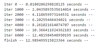
for i, rowi in df.iterrows():
# 매 1000번째 반복마다 경과 시간을 출력합니다.
if i % 1000 == 0:
print(" iter {} -- {} seconds --".format(i, time.time() - start_time))
# 영화 노드 추가
G.add_node(rowi['title'], key=rowi['show_id'], label="MOVIE", mtype=rowi['type'], rating=rowi['rating'])
# 영화의 배우들과의 관계 추가
for element in rowi['actors']:
G.add_node(element, label="PERSON")
G.add_edge(rowi['title'], element, label="ACTED_IN")
# 영화의 카테고리와의 관계 추가
for element in rowi['categories']:
G.add_node(element, label="CAT")
G.add_edge(rowi['title'], element, label="CAT_IN")
# 영화의 감독과의 관계 추가
for element in rowi['directors']:
G.add_node(element, label="PERSON")
G.add_edge(rowi['title'], element, label="DIRECTED")
# 영화의 국가와의 관계 추가
for element in rowi['countries']:
G.add_node(element, label="COU")
G.add_edge(rowi['title'], element, label="COU_IN")
# 유사한 영화 찾기
indices = find_similar(tfidf, i, top_n=5)
snode = "Sim(" + rowi['title'][:15].strip() + ")"
G.add_node(snode, label="SIMILAR")
G.add_edge(rowi['title'], snode, label="SIMILARITY")
# 유사한 영화들과의 관계 추가
for element in indices:
G.add_edge(snode, df['title'].loc[element], label="SIMILARITY")
# 처리가 완료되었음을 출력합니다.
print(" finish -- {} seconds --".format(time.time() - start_time))
6. 두 개의 영화를 살펴보기
def get_all_adj_nodes(list_in):
# 주어진 영화 목록과 연결된 모든 노드를 가져오는 함수
sub_graph = set()
# 주어진 영화 목록에 대해 반복
for m in list_in:
sub_graph.add(m)
# 각 영화와 연결된 모든 노드를 가져옴
for e in G.neighbors(m):
sub_graph.add(e)
# 리스트로 변환하여 반환
return list(sub_graph)
def draw_sub_graph(sub_graph):
# 부분 그래프를 생성합니다.
subgraph = G.subgraph(sub_graph)
colors = []
# 노드의 라벨에 따라 색상을 지정합니다.
for e in subgraph.nodes():
if G.nodes[e]['label'] == "MOVIE":
colors.append('blue')
elif G.nodes[e]['label'] == "PERSON":
colors.append('red')
elif G.nodes[e]['label'] == "CAT":
colors.append('green')
elif G.nodes[e]['label'] == "COU":
colors.append('yellow')
elif G.nodes[e]['label'] == "SIMILAR":
colors.append('orange')
elif G.nodes[e]['label'] == "CLUSTER":
colors.append('orange')
# 부분 그래프를 시각화합니다.
nx.draw(subgraph, with_labels=True, font_weight='bold', node_color=colors)
plt.show()
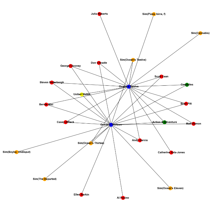
# 주어진 영화 목록에 대해 부분 그래프를 그리는 함수 호출
list_in = ["Ocean's Twelve", "Ocean's Thirteen"]
sub_graph = get_all_adj_nodes(list_in)
draw_sub_graph(sub_graph)
"Ocean's Tweleve"와 "Ocean's Thirteen" 영화의 sub-graph를 그려봤다.
7. 추천 함수
def get_recommendation(root):
    # 공통 이웃을 저장하는 딕셔너리 생성
    commons_dict = {}
    # 주어진 영화의 이웃을 반복
    for e in G.neighbors(root):
        # 이웃의 이웃을 다시 반복
        for e2 in G.neighbors(e):
            # 자기 자신은 제외
            if e2 == root:
                continue
            # 이웃이 영화인 경우
            if G.nodes[e2]['label'] == "MOVIE":
                commons = commons_dict.get(e2)
                # 공통 이웃 딕셔너리 업데이트
                if commons == None:
                    commons_dict.update({e2: [e]})
                else:
                    commons.append(e)
                    commons_dict.update({e2: commons})
    # 추천할 영화와 가중치를 저장할 리스트 생성
    movies = []
    weight = []
    # 공통 이웃 딕셔너리를 순회하면서 가중치 계산
    for key, values in commons_dict.items():
        w = 0.0
        # 이웃의 가중치를 계산하여 합산
        for e in values:
            w = w + 1 / math.log(G.degree(e))
        # 영화와 가중치를 각각의 리스트에 추가
        movies.append(key)
        weight.append(w)

    # 결과를 Series로 변환하여 가중치에 따라 정렬
    result = pd.Series(data=np.array(weight), index=movies)
    result.sort_values(inplace=True, ascending=False)
    return result;
추천 함수는 맨 위에서 설명한대로 이웃 노드를 가장 많이 공유하고 있는 노드들을 계산하는 방식이다.
예를 들어 내가 A라는 영화를 입력으로 주었으면, A라는 영화(노드)과 이어진 다른 노드들에 가장 많이 이어져있는 영화 노드를 찾는 것이다.
8. 추천 받기
# 각 영화에 대한 추천 목록을 가져옵니다.
result = get_recommendation("Ocean's Twelve")
result2 = get_recommendation("Ocean's Thirteen")
result3 = get_recommendation("The Devil Inside")
result4 = get_recommendation("Stranger Things")

# 각 영화에 대한 추천 목록을 출력합니다.
print("*"*40+"\n Recommendation for 'Ocean's Twelve'\n"+"*"*40)
print(result.head())
print("*"*40+"\n Recommendation for 'Ocean's Thirteen'\n"+"*"*40)
print(result2.head())
print("*"*40+"\n Recommendation for 'The Devil Inside'\n"+"*"*40)
print(result3.head())
print("*"*40+"\n Recommendation for 'Stranger Things'\n"+"*"*40)
print(result4.head())
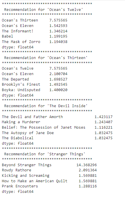
Recommendation for "Ocean's Twelve":
"Ocean's Thirteen"이 가장 높은 가중치인 7.575565를 가진다. 이는 "Ocean's Twelve"와 "Ocean's Thirteen" 사이의 유사성을 나타낸다.
그 외에도 "Ocean's Eleven", "The Informant!", "Babel", "The Mask of Zorro" 등의 영화들이 추천 목록에 있는것을 볼 수 있다. 이 추천 목록은 "Ocean's Twelve"와 유사한 성격이나 스타일을 가진 영화들을 나타낸다.
Recommendation for "Ocean's Thirteen":
"Ocean's Twelve"가 가장 높은 가중치를 가진다. 이는 "Ocean's Thirteen"과 "Ocean's Twelve" 사이의 유사성을 나타낸다.
그 외에도 "Ocean's Eleven", "The Departed", "Brooklyn's Finest", "Boyka: Undisputed" 등의 영화들이 추천 목록에 있다.
이 추천 목록은 "Ocean's Thirteen"과 유사한 성격이나 스타일을 가진 영화들을 나타낸다.
Recommendation for "The Devil Inside":
"The Devil and Father Amorth"가 가장 높은 가중치를 가진다. 이는 "The Devil Inside"와 "The Devil and Father Amorth" 사이의 유사성을 나타낸다.
그 외에도 "Making a Murderer", "Belief: The Possession of Janet Moses", "The Autopsy of Jane Doe" 등의 영화들이 추천 목록에 있다.
이 추천 목록은 "The Devil Inside"와 유사한 주제나 스타일을 가진 영화들을 나타낸다.
Recommendation for "Stranger Things":
"Gossip Girl"이 가장 높은 가중치를 가진다. 이는 "Stranger Things"와 "Gossip Girl" 사이의 유사성을 나타낸다.
그 외에도 "Breaking Bad", "Kicking and Screaming", "How to Make an American Quilt", "Prank Encounters" 등의 영화나 TV 프로그램들이 추천 목록에 있다.
이 추천 목록은 "Stranger Things"와 유사한 장르나 분위기를 가진 작품들을 나타낸다.
이 추천 목록들은 각 영화의 특성과 유사한 작품들을 추천하고 있다.